MATLAB in the Biosciences - a Tutorial
The aim of this tutorial is to provide people working in the biosciences with little to no background in programming an accessible and short tutorial on MATLAB basics for common bioscience workflows. It was developed for some courses here at the EMBL and includes exercises plus solutions (or download as pdf), though as the data are as of yet not included in this blog post, it will not really be possible to work through these exercises. MATLAB release 2013a was used for this tutorial, it will most likely differ considerably from other, especially earlier releases. If you have any questions or comments, feel free to email me.
MATLAB syntax and data types
All subsequent commands need to be entered in the MATLAB command line.
Variables store values under a variable name
a = 5
Semicolons suppress printing of outputs
b = 6;
who and whos provide information about variables
who
whos a
Floating point values are of the data type single or double (double is the default variable type in MATLAB)
c = 5.5
a+c
ans is always the last result if the result of a command has not been assigned to a variable
whos ans
MATLAB can be used as a calculator with *,/ and ^ denoting multiplication, division and potentiation, respectively
b*c
b/c
b^c
MATLAB understands scientific notation (10^-5 == 1e-5)
0.00001 == 1e-5
MATLAB stands for MATrix LABoratory and is specialized for the handling of vectors and matrices. Vectors are specified using brackets
a = [1 2 3 4 5]
b = [3 4 5 7 8]
Vectors can be added and multiplied (this * multiplication is a dot or scalar product!)
a+b
a*b % does not work, as this is a
% vector dot product and requires that
% vector dimensions agree
You can get information on the dimensions of a vector using
size(a), size(b), length(a)
Element-wise multiplication and division work by putting a . in front of *, / and ^
a.*b % works
a./b
' is the transposition operator that converts a row vector into a column vector and vice versa
b'
Operators can be combined and used in this example to get a valid dot product
a*b' % now that works as well
%  and returns the scalar product
Operators are evaluated in the following order (more about these unknown operators later)
- Parentheses
()- Transpose (
'), power (.^), complex conjugate transpose ('), matrix power (^)- Unary plus (
+), unary minus (-), logical negation (~)- Multiplication (
.*), right division (./), left division (.\), matrix multiplication (*), matrix right division (/), matrix left division (\)- Addition (
+), subtraction (-)- Colon operator (
:)- Less than (
<), less than or equal to (<=), greater than (>), greater than or equal to (>=), equal to (==), not equal to (~=)- Element-wise AND (
&)- Element-wise OR (
|)- Short-circuit AND (
&&)- Short-circuit OR (
||)
The colon operator : allows you to create a vector by incrementation
i = 1:10 % increment by one
ij = 0:0.1:2*pi % increment by 0.1
Elements and slices can be extracted from a vector by indexing
a(1) % extract the first element from vector a
a(5) % extract the fifth element from vector a
a(end) % extract the last element
For those of you familiar with C, Java or Python (or many others), MATLAB indices start at 1, not at 0 as in the other languages.
The colon operator : can be used to create vectors; vectors can be used to index into vectors:
a(1:3) % extracts the elements
% 1:3 == a([1 2 3])
a(2:end-1) % extracts the elements
% a([2 3 4 ... end-1])
To build a column vector, use ; to denote the next row
colvec = [1; 2; 3; 4]
... enables multiline expressions in MATLAB
colvec = [1;...
          2;...
          3;...
          4]
Matrices are created by combining row and column vector notations
A = [1 2 3; 4 5 6; 7 8 9]
A(1,1)
A(2,3)
A(1:3,1:2)
A(:,1:2)
A([1 3],[2 1]) % slicing into matrices
% requires providing two indices
A' %  the transpose operator

B=rand(3,3) % a number of functions
% exist to create special vectors
% matrices (rand: random uniform numbers)
size(A), length(A), numel(A)
% get the number of elements of a vector or matrix
A*B % the normal multiplication
% operator * performs a matrix multiplication
% (C(1,1) = A(1,1)*B(1,1) + A(1,2)*B(2,1) + A(1,3)*B(3,1)...)
A.*B % the dot multiplication operator
% .* performs an element-wise multiplication
% (C(1,1) = A(1,1)*B(1,1)...)
A+B % the addition operator does not
% care whether it should add scalars,
% vectors or matrices (you don't need to
% loop through an array to add each element)
Matrices and vectors with the right dimensions can be concatenated
[A B] % creates a 3 x 6 array
[A; B] % creates a 6 x 3 array
[A; a] % concatenates a matrix with
% a vector and creates a 4 x 3 array
A number of specialized functions can be used to create arrays and vectors
zeros(5) % 5 x 5 array of zeros
ones(5,4) % 5 x 4 array of ones
eye(5) % 5 x 5 identity matrix
rand(5,3) % 5 x 3 matrix of
% random numbers
t=linspace(0, 10,50); % vector of
% 50 equally-spaced numbers between 0 and 10
tl=logspace(-4,-1,50); % vector of
% 50 logarithmically spaced values
% between 1e-4 and 1e-1
A huge number of general math functions exist, e.g.,
round(t) % rounds to the nearest integer
ceil(t) % rounds to the upper integer
floor() % rounds to the lower integer
Trigonometric functions work just as expected
sin(t)
cos(t)
Exercise 1
- Create a
3 x 3matrixAand a3 x 1vectorb- Multiply
Awith the first element ofb- Multiply
Aandb- Concatenate
bwith itself 2 times to get a3 x 3arrayB- Multiply
AandBelement-wise to getA- Extract: row
2, column1; row3, all columns; rows2,3columns2,3
Relational Operators compare values and return boolean values (true == 1 or false == 0)
a>2
b~=3, B==2
A>2 & B==3
When using relational operators on vectors or matrices, logical arrays (arrays of 1s, where the relation is true and 0s where the relation is false) are returned. Logical arrays can also be used to index into other arrays
r1=round(5.*rand(10,1))
r2=round(5.*rand(10,1))
l = r1==r2 % create a logical
% array the same size as r1
r1(l) % extract those elements
% of r1 that are true for the previous relation
~l % use the negation operator
% to flip the logical array
r1(~l) % extract those elements of
% r1 that are false (!) for the previous relation
find(l) % find() returns the indices
% of the true values in a logical array
find(r1>3) % find can be combined with
% operations that return logical arrays

floor(r1), ceil(r2)
A(A>2 & B==3) % indexing with logical arrays
Exercise 2
- Create a vector
tfrom0to2 piof size100- Compute the sine (
sin()), assign totnew- Compute the arcsine of
tnew, assign to new vectortc(useasin())- Test whether
tcandtare equal- Find the elements in
tandtcthat are not equal (usingfind()or logical indexing)
How to get help
- Tab completion, Function hints
help rand
-
functionname + F1
-
if function is unknown, click on fx, search
doc rand
- Help on the web: MathWorks Docs, MATLAB Answers, Stack Exchange/Stack Overflow
- Tech Support (available from within the MATLAB Desktop)
Exercise 3
- For the vector
tnew, compute the maximum, minimum, absolute value- For the vector
t, compute the square root and the base 10 logarithm
Strings and cell arrays
MATLAB uses only single quotation marks for strings
s = 'embl' % creates a character array
s(2) % you can index into the character
% array just the way you learned it before
s(2:4)

s2 = 'European…'
s3=[s s2] % character arrays can be
% concatenated (i.e., one put after the other)
s3=='e' % character arrays support equality operators
s3=='E'

strcmp(s,s3) % strcmp compares character arrays
strncmp(s,s3,4) % strncmp requires the number of character to be compared

s4 = ['embl'; 'dkfz'] % character arrays can be vertically concatenated ('stacked') if the dimensions agree
s4(2,1:3)
Cell arrays are data structures or containers that can hold a variety of different data types (such as numerical data and strings etc.). They are especially useful to hold many strings with differing lengths
s4 = {'embl'; 'dkfz'} % use curly
% braces to build a cell array
s4(2) % index into cell arrays
% - this will extract the second
% element, which is 'dkfz'!
s4{2} % two different indexing notations
% exist for cell arrays: parentheses extract
% the elements as cell arrays,
% curly braces access the content -
% this will extract a string

s4{3} = ones(5) % mix strings and numerical data
s4{1,2} = rand(4)
s4{1,2}(1,3) % use nested indexing to
% access array elements inside the cell array
Regular Expressions are powerful tools to systematically analyze strings
s='European Molecular Biology Laboratory 2013'
regexp(s,'\d') % patterns in strings can
% be found and extracted using regular
% expressions: '\d' finds numbers
regexp(s,'\d','match') % 'match' returns
% the matching part of the string
regexp(s,'\d*','match') % quantifiers are
% used to extract more than one matching element
regexp(s,'[A-Z]','match') % character ranges
Exercise 4
- Create a string variable with your name
- Make it all upper case, lower case
- Add a second string ‘EMBL’ as a cell array
Structures
Structures are another container format for heterogenous data. Structures contain fields which allow you to access data by using a meaningful field name
institute = struct('Name','EMBL','Age',39); % create
% a structure containing the two fields Age and Name
institute.Name
institute.Location = 'Heidelberg' % add a third field

institute(2).Name = 'EBI' % structures can
% be arrays (or 'arrays of structures')

institute(2).Age % the element exists but is empty
institute(2).Age = 18;
institute(2).Location = 'Hinxton';

[institute(:).Age] % put all 'Age' elements into an array
Saving variables
save % saves all variables in the current
% workspace in matlab.mat
save data.mat var1 var2 ... % saves only
% the specified variables
A complete Data Analysis Workflow
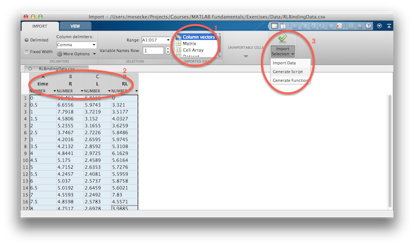
To get you started with the MATLAB Desktop, I will introduce a couple of GUIs that are part of the Desktop and will allow you to create and automate a data analysis workflow without needing to code anything yourself. The data are available from a csv file called 'RLBinding.csv'. Navigate to the folder where this is located, then simply double-click on the file in the 'Current Folder Browser' and, at least from about release 2012b onwards, the 'Import Tool' will open. The same would happen with, e.g., Excel files. Choose to import the data as column vectors (1 in the screenshot below). Other options are to import the data as a matrix, cell array or as a dataset array. Next, rename the columns to whatever you wish the imported vectors to be named (2). Finally, generate a script or function (3) using the code generation facility and import the data into the workspace. Upon generating a script or function, an editor window will open and you will have to save the file (e.g., as importdata.m in the case of a generated function).
Next, we plot the data using interactive tools. Open the 'Workspace Browser', choose the variables to be plotted (e.g., time and R) and head to the 'Plot' tab. Choose the first option 'plot'. A figure window will open up, similar to the one in the centre of the image below.
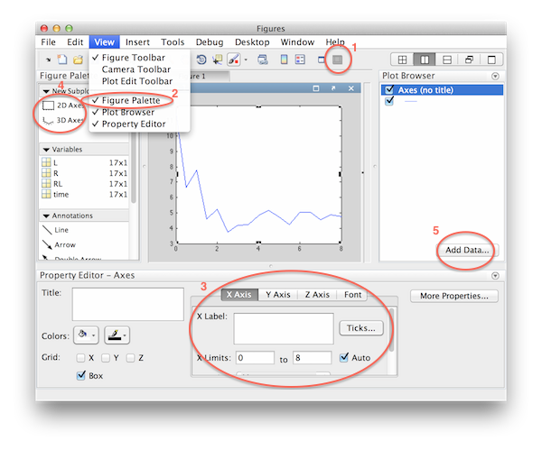
Open the 'Plot Editor Tool' (1) and another GUI will open that can be used for any modification of the plot. If anything, e.g., the 'Figure Palette' is not displayed, head to the 'View' menu and tick the appropriate items (2). The 'Property Editor' (3) displays different items depending on the active element in the plot (click to change) and enables you to change any property of the plot. Add new 2D and 3D subplots using the 'Figure Palette' (4). Add additional lines to the plot by using the 'Add Data' button (5). By default the 'X Data Source' is set to 'auto', change that to the actual x-axis data (e.g., 'time'). Once you edited the plot according to your tastes, go to 'File->Generate Code' and another function will open up in the editor that can be used to precisely reproduce the plot automatically, for example, for new data sets. The last step is to save the plot in a format that could be used in a publication, tiff or eps, for example. Go to 'File->Export Setup' to save the plot in a format and resolution of your choice. However, I strongly dislike this dialog and would always prefer going through either the print command or the excellent export_fig function available from the MATLAB File Exchange.
Exercise 5
Use the interactive tools in the MATLAB Desktop to:
- Import the data in
RLBinding.csvas column vectors (time,R,L,RL). Generate and save code- Plot the data using diamonds/circles/crosses and dotted lines
- Change the
LineWidthto2.5,Colorto something else- Add labels and a title. Generate and save code
- Export (
Scripts
Scripts store a list of commands in a single file. The file name needs to end with .m. Execute a script by typing the file name in the command line or by clicking the run button. A script is similar to running each line separately in the command line, however, it can be helpful for the automation of repetitive tasks.
It is best to describe in a script what each line does; MATLAB uses % for comments: Everything after % is neglected when executing a script. The MATLAB Desktop has a second functionality called cell mode which uses double percentage signs %% to structure a script into separate executable sections. Hit Run section to execute only the currently active cell.
Exercise 6
- Combine the commands from Exercise 5 into one script a. import b. plot
- Save it as
plotdata.m- Add
%and%%comments that explain what you are doing- Use the
publishbutton to create a pdf report
Control Flows
Suppose you want to repeat a certain calculation over and over or you want to change a small part of your program depending on some variable. This is what control flow commands are used for. Two major repetition blocks are available in MATLAB, for and while. for requires a vector of monotonically increasing numbers and executes the code between for and end for each of the numbers in said vector.
for ii = 1:5
    sprintf('The current value is %d\n',ii)
end
The while loop repeatedly executes a code block while a condition is met. It can be used in a similar fashion to the for loop by using an incremented variable inside the while block. The key difference to the for loop is that the for loop is always executed at least once; the while loop can also be not executed at all.
k = 1;
while k <= 5
    sprintf('The current value is %d\n',k)
    k = k + 1;
end
if tests whether a condition is true or not; if the condition is true, the code block following the if is executed. elseif tests whether another condition is true and conditionally executes its code block. The else block is executed when no condition is true.
checkcondition = 10;

if checkcondition <= 5,
    plot(rand(5))
elseif checkcondition > 10,
    plot(sin(0:0.1:2*pi))
else
    disp('Nothing happens')
end
Similar to if, the switch/case construct allows you to conditionally execute code. However, in this case it is best used for string matching, i.e., in a situation where you want to switch the program behavior due to some flag that you provide.
t = 0:0.1:2*pi;
flag = 'sin'

switch flag
    case 'cos'
        plot(t,cos(t))
    case 'tan'
        plot(t,tan(t))
    case 'sin'
        plot(t,sin(t))
    otherwise
        disp('Please provide a plot type')
end
Exercise 7
- Take the previous script called
plotdata.mand usefiles = dir('*.csv')to get a list of allcsvfiles in the current folder- Use a
fororwhileloop to create a subplot for the data in each of the different files
Debugging
Sometimes, or maybe very often, MATLAB will error or not show the right results when you are running your own function or script. This is where the debugger comes in handy. The debugger allows you to execute the code to a certain point (the breakpoint) and then explore the values of the variables, run alternative code or step through the code to see how the variables change. The MATLAB Editor has a set of GUI elements to control the Debugger; from the command line, the following commands are equivalent to the GUI elements.
dbstop in filename at 127 % sets a
% breakpoint at line 127 in file filename
dbstop if error % starts the debugger
% if an error exception occurs

dbstep % once in debugger mode, dbstep
% let's you step to the next line - the
% current line is executed
dbstep 10 % executes 10 lines and then
% stops
dbcont % let's the function continue
% (either to the next debugging point or
% to the end of the function)
Mathematical Modelling of Biological Systems
(a really short primer)
Mathematical Modelling is a subject that could be - and will be - its own course. Modelling can be used for a wide variety of purposes, to mention just a few:
- Formalization of mental models. Everyone has a mental model of his subject of research that represents the beliefs in the causal connections between different items such as proteins. However, such as model is difficult to communicate precisely to others and prone to fail when complex nonlinear relationships need to be included. Formalizing such a mental model into a mathematical model enables its direct validation using quantitative predictions and experiments and provides a tool to communicate and critically discuss one's beliefs about a system.
- Prediction or Forecasting. See, e.g., the weather forecast. Foreseeing previously unobserved behaviors is a crucial method to confirm the validity of a model and through that of a hypothesis. Prediction is also an essential tool for control: Given current conditions of a process, which parameters need to be tweaked to guide the system into a wanted direction? Controling the differentiation of stem cells into a certain cell type by timed addition of transcription factors is one (hypothetical) use case.
- Optimization of Production. Suppose you are using a cellular system to produce a given product. One approach to increasing the production is to randomly create strains and select for the best producer; another is to combine this approach with artificial evolution. These approaches can be combined with rational design of strains using mathematical modelling where the relevant system parts are modelled and mathematically optimized to overproduce the wanted product.
- Design of Experiments. A typical approach in biological experiments, especially in time series experiments, is to measure some system element (that one deems important) at equidistant time points. However, it is in no way guaranteed that this will provide informative data sets. Mathematical Modelling can be used to predict measurement points that will provide the most information.
Modelling, modelling formalisms and modelling methods will be the topic of another course. Here, I will limit this section to Ordinary Differential Equations (ODEs) as they are the most ubiquitous modelling method.
Ordinary Differential Equations
The most basic ODE describes radioactive decay or the self-inactivation of GTPases like Ras. The rate of change in the concentration (here: $x$) is simply depending on its own concentration at any given point in time multiplied by a constant:
$$\frac{dx}{dt} = - k x$$
The solution $x = f(t)$ to this is easy to find: we are looking for a function whose derivative reproduces itself up to a constant factor
$$x = C e^{-k t}$$
C is given by the initial conditions of this equation, e.g., $x_0$. A similar equation describes bacterial growth in the absence of substrate limitations
$$\frac{dx}{dt} = \mu x$$
The solution to this is exactly the same as before, with the exception that the exponent is not negative
$$x = C e^{\mu t}$$
These are simple equations, readily solvable by standard methods for linear differential equations. Few equations governing biological behaviors are as simple as that. For example, bacterial growth in the presence of substrate limitations is modeled by the Monod equation (which is very similar to the Michaelis-Menten equation in enzyme catalysis)
$$\frac{dx}{dt} = \frac{\mu_{max} s }{(K_s + s)} x$$ $$\frac{ds}{dt} = - \frac{1}{y_{xs}}\frac{\mu_{max} s}{(K_s + s)} x$$
where $s$ is the substrate concentration. The solution to this is much harder to find and involves the Wright $\omega$ function, a function that cannot be represented by elementary functions. Most equations describing biological systems are too nonlinear to be solvable analytically.
However, it is possible to solve any equation numerically, i.e., by substituting numbers into the equation and iteratively updating the resulting function values. One method to compute a solution, though obsolete nowadays, is the Euler method. It is based on the following idea: We know the derivative of the unknown function $x = f(t)$ as it is just the right hand side of our ODE $\frac{dx}{dt} = f(x,x',...)$. At any point of the solution this equals the difference $\Delta x/\Delta t$ and is tangential to the solution. If we now define a step h as a freely chosen $\Delta t$, we can calculate the $\Delta x$ by computing $\Delta x = f(x,x',...) h$. Starting from the initial condition $x_0$, an iterative solution can be found using the following iteration rule:
$$x_{i+1} = x_i + f(x,x',...) h$$
The error of this algorithm depends strongly on the value of $h$; due to its limitations, the algorithm has been largely superseded by other methods such as Runge-Kutta. MATLAB provides a number of different ODE solving algorithms that are adapted to different problems. The basic function signature for ODE solvers is
[t,x] = odesolver(@odefun, tspan, x0, options)
where @odefun is a function accepting exactly two arguments, t, x, and returning one argument, the derivative dx/dt.
Functions
Functions are used to store several commands in a single file and separate the variables from other code blocks so that no name collisions occur.
They accept a list of input arguments (here: in1, in2) and return a list of output arguments (here: out1, out2). Functions are great if you want to reuse an algorithm again and again (e.g., to calculate the mean). In MATLAB, function names and file names must be identical.
function [out1, out2] = functionName(in1, in2)
% comments directly after the function declaration
% are shown when 'help' and 'doc' are used

% commands go in here

    function [nestedOut] = nestedFunction(nestedin)

        % nested Functions have access to variables
        % in the parent function, but the parent function
        % does not have access to variables in the nested
        % function

    end

end

function [hiddenOut] = hiddenFunction(in)

    % this function is only visible for the functions
    % inside this file

    % when using nested functions or several
    % functions per file, each function block must
    % be ended with 'end'

end
Scope
Scope refers to the visibility of functions and variables. Functions are only visible when they are on the Path: a list of folders that MATLAB searches when you type a function name. The current folder . is always on the path.
Only the main function (the first function in a file, i.e., the file name) in a file is accessible from outside functions (functions in different files). A single file can contain any number of functions, though it is typically best to have fewer functions per file, at least in MATLAB. The additional functions can only be accessed from within the primary function.
Variable Scope refers to the visibility and accessibility of variables. When executing a script, for example, all the variables reside in the workspace and are visible for all commands in the command line. When running a function, however, the function cannot access the variables in the workspace (except if you explicitly called the function with said variables as input arguments) and the variables inside the function block are inaccessible from the outside. This is also important for functions inside a file. In the example above, one function is inside another function's block (demarked by function ... end), another function is outside said function block. The first one is called a nested function. If a variable is defined at the same time in the parent function and the nested function and the variable is not added as an input argument to the nested function, the nested function can access and modify this variable. This helpful feature will be used later in the parameter estimation example. The function outside the main function block, however, does not have access to the variables inside the parent block.
Exercise 8
- Build an ODE system model for the
R + L -> RLreaction withkfas the forward reaction rate- Create a function
oderhs.mthat accepts two argumentstandxand returns the value of the derivative for each value oftandx- Create a function
odeeuler.mthat implements the Euler method to compute the numerical solution of theR+Lsystem- Solve the ODE system in
oderhs.musingodeeuler.mand plot the solution for different values of $h$
Parameter Estimation
Very often the actual parameter values of a model of a biological system are unknown or imprecisely known: direct measurements are often impossible and in vitro measurements are weak representations of cellular realities. It is therefore necessary to estimate the parameters from experimental data. In the case of an ODE, this requires two steps as we want to fit the numerical simulations to the experimental data. The first step is to compute a numerical approximation to our system; we just explored that. The second step is to compute a measure that describes the deviation of the simulation from the experimental data and minimize this deviation. A classic metric is Least Squares (LSQ),
$$LSQ = \frac{1}{n-1} \sum_i{\sqrt{(x_{d,i} - x_{p,i})^2}}$$
where $x_{d,i}$ is the $i$th data point and $x_{p,i}$ is the corresponding simulated value. As $x_{p,i}$ depends on the parameters $\theta$ of the model, the $LSQ$ is also a function of the parameters: $LSQ = f(\theta)$. The parameters $\theta$ can include the initial conditions of the system. The aim now is to find parameters $\hat \theta$ that minimize $LSQ$.
This multivariate nonlinear optimization problem can be solved using the wide range of algorithms developed for these problems. These algorithms can be classified into two classes: deterministic (or local) and heuristic (or global). A key difference between these two classes is reproducibility: restarting a deterministic algorithm with exactly the same conditions will lead to exactly the same results; the heuristic algorithm depends on random values and will often return a different result. Furthermore, local algorithms exploit derivative properties of the objective function such as Jacobians or Hessians to iteratively identify possible next solutions; global algorithms are very often modeled after some natural process that finds optimality of a certain natural problem: for example, ant colony optimization as well as particle swarm optimization use many parallel searchers with interaction to find optimality, similar to how ants crowd-source finding the optimal path to a food cache. Other examples include evolutionary programming and genetic algorithms, where, as the name implies, optimality-finding biological processes are used as templates. Despite their name, global optimization algorithms cannot guarantee to find the unique global solution; however, in practice, the obtained results are often good enough to continue with the model exploration.
In MATLAB, both local as well as global optimization algorithms are available. The Optimization Toolbox offers the former, while the latter are available in the Global Optimization Toolbox. The typical function signature for Optimization toolbox algorithms is
optimsolver(@minimfun, theta0, ...)
@minimfun is a function that accepts parameter values and returns the metric to be minimized. Therefore, we need to write a function that accepts only parameter values and returns the least squares value. This is best achieved by using a nested function so that experimental data are accessible to the minimfun.
Exercise 9
Use the model and the data to learn the parameters of the system:
- Write a function
objfunction.mthat contains the data, accepts a vector of parameter values and returns the LSQ term- Extend the function so that it (i) reads in the data once, (ii) calls
lsqnonlinusing the previousobjfunction, now nested, to provide the function value to be minimized and (iii) calculates the best parameter fit
Image Processing with MATLAB
(another really short primer)
Images are matrices: A rectangular table containing intensities (in a variety of formats) of each pixel. The most usual format is based on 8 Bit and can therefore distinguish 256 different colors. The Red-Green-Blue (RGB) system has 8 Bit intensity values for each of the three colors (commonly referred to as 24 bit RGB) and can therefore encode more than 16 million colors. A large variety of image formats exist. The most used format in biological applications is probably the TIFF (Tagged Image File Format) format, which allows for lossless storage (unlike, e.g., jpeg). However, TIFF can also be used as a container to store jpeg and other compressed image formats. Until recently, TIFF files were limited to 4GB; this limitation has recently been lifted and MATLAB is able to read bigTIFFs since release 12b.
In the following workflow, we will read in TIFF images, compute the maximum intensity projection, interactively explore the image, segment the image using a simple thresholding operation and finally identify cells to count them.
Importing TIFF images into MATLAB
ims = imfinfo('Img1.tif') % get some informations about the image

% the image is a multiframe image: the first image is DIC, the
% second is fluorescence. We need to extract the image size and
% read in every second image plane into the preallocated array

% preallocate an array the size of the image
imstack = zeros(ims(1).Height,ims(1).Width, length(ims));

% First, we read in all 42 images in the file
for ii=1:length(ims)
    imstack(:,:,ii) = imread('Img1.tif','Index',ii);
end

% then we split the image stack into two parts -
% the first 21 images are the fluorescence channels,
% the second 21 images the DIC channels

imstackf = imstack(:,:,1:end/2);

% let's explore the images a bit
size(imstackf)
imstackf(1:10,1:20,1)
max(imstackf(:)) % expore the value range
% (or intensity range) for the image
min(imstackf(:))
Enhancing the image
imm = max(imstackf,[],3); % calculate
% the maximum intensity
% projection - simply use max() along the
% third dimension (the stack)

img = mat2gray(imm); % convert the image
% to a grayscale image that has a range of [0,1]
img(1:10,1:20,1)

imtool(img) % imtool is a special GUI in
% MATLAB that allows you to interactively
% explore images (zoom, explore pixel values etc.)

ims = imsharpen(img); % sharpen the image
% by subtracting a blurred version of the image
imtool(ims)
Image Segmentation
threshold = graythresh(ims) % an automatic
% way of calculating a threshold
% for the subsequent segmentation

imthresholded = im2bw(ims,threshold); % the
% simplest segmentation method:
% everything above the threshold becomes
% 1 (white), everything below the threshold
% becomes 0 (black)

subplot(1,2,1),imshow(img),subplot(1,2,2),imshow(imthresholded)

imfilled = imfill(imthresholded,'holes');
% some parts inside the cell are above
% threshold, the imfill function fills all
% holes (which are image segments of ones
% completely surrounded by zeros)
imtool(imfilled)

imobjs = bwlabel(imfilled) % identify and
% enumerate all objects - the output matrix
% will have 1s at the first object, 2s at
% the second object etc.

labeledim = label2rgb(imobjs); % convert the
% label matrix to an RGB image which
% can be used to visually see the different identified objects
imshow(labeledim)
Extracting Object properties
One of the aims of automatic image processing is to extract quantitative information from a large number of images without any (or many) manual steps. regionprops is a powerful function to extract a large number of statistics for the objects in an image, e.g., Area, the area of the object, Perimeter, the perimeter of the object, MajorAxisLength for the length of the major axis of the enclosing ellipsis and Orientation for the angle between the major axis and the x-axis.
improps = regionprops(imobjs,'all') % one of
% the most powerful tools of the Image
% Processing Toolbox: regionprops calculates
% a large number of statistics
% (check the docs for the full list) for each object.
One of the properties regionprops returns are indices of the objects which can be used to directly extract that subimage. As we binarized the image to find the cells, this image has the same size and the locations as the original image and we can use the region properties of the segmented image to explore the original grayscale image, img. SubArrayIdx can be used to extract the subimages.
firstObj = img(improps(1).SubarrayIdx{1}, improps(1).SubarrayIdx{2});
imshow(firstObj)
imsize = size(firstObj);

% plot the central profile of the cell
plot(firstObj(round(imsize(1)/2),:),'k.','MarkerSize',6)
% plot the whole cell as a surface
surf(firstObj,'FaceColor','interp','EdgeColor','interp')

% we can now compare the intensity profiles for
% all the objects in this image by looping over the number
% of identified objects and then plotting
% the surfaces in subplots

% first, figure out how many rows and
% columns we need to display the surfaces
nobjs = length(improps);
nrows = round(sqrt(nobjs));
ncols = ceil(sqrt(nobjs));

% loop through the images and plot them into individual subplots
for jj = 1:nobjs
    obj = img(improps(jj).SubarrayIdx{1}, improps(jj).SubarrayIdx{2});
    subplot(nrows, ncols, jj), surf(obj,'FaceColor','interp','EdgeColor','interp')
end
Exercise 10
Write a script that
- Reads in all images in the ‘Images’ folder (
forloop)- Reads in all fluorescent images in the tiff file (another
forloop)- Computes a maximum intensity projection for each file
- Computes a threshold
- Uses the threshold for segmentation
- Calculates the number of cells in each image using regionprops
- Optional: Use a subplot to do a
surf()plot of every first object in each image file