Julia for MATLAB users I

A number of excellent free open-source alternatives to MATLAB have arrived in the last couple of years that have managed to bite away parts of MATLAB's market share. Most notable are R, which is now the dominant language for statistical computing and bioinformatics and Python (with numpy, scipy etc.) which, as a general-purpose language, delivers a great integrated experience - it is great for scientific computing and, e.g., web development at the same time. However, none were really able to replace MATLAB completely, which is probably due to how MATLAB hides complexity from its users and how it provides easy to use mathematical functions as well as powerful libraries (toolboxes in MATLAB speak) that are available (for a cost).

A potential contender sprang to life last year, julia. Julia intends to combine the best from MATLAB, R and Python into one language that is supposed to be consistent, well designed and most importantly fast. The julia people show some impressive benchmark stats on their website. I wanted to explore julia as a possible replacement for MATLAB. The simplest thing that I'm doing in MATLAB and one of the workflows I'm always showing in courses at EMBL is some very basic data visualization:

1. Read in data stored in a csv file
2. Plot the data
3. Export the plot

This is straightforward to do in MATLAB and relatively straightforward in julia. However, we need to set up julia and some of its packages first, which is less straightforward. I published a guide here. What's important is that we added two of the three major plotting packages for Julia, Winston and Gadfly. Let's start with how things are done in MATLAB. In this comparison I will follow two different approaches in both languages, (i) importing data into a standard array and then plotting it and (ii) importing data into a heterogenous data container (dataset/table in MATLAB, dataframe in julia) and then plotting it. The use of the second approach is described in part iii of this series.

First approach: standard arrays in MATLAB

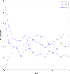
% The data in the file contain synthetic 
% receptor-ligand binding time series data
rldata = csvread('rlbinding.csv'); % reads in comma-separated csv file
% use dlmread('rlbinding.csv','\t') if you have tab-delimited files

% separate data into different vectors
t = rldata(:,1); R = rldata(:,2); L = rldata(:,3); RL = rldata(:,4);

The data can be plotted into a single plot or into several different tiled plots using subplot (see part ii of this series):

% single plot   
plot(t,R,'-bd',t,L,'-bo',t,RL,'-bx','MarkerSize',8)
legend({'R','L','RL'})
xlabel('time')
ylabel('concentration')

The resulting figures can be exported using the base MATLAB print command (which I cannot stand) or the File Exchange submission export_fig (which I can highly recommend)

% png output in 72 dpi resolution
export_fig('matlab_rlbinding.png','-png', '-r72','-transparent')

Using standard arrays in julia

Let's have a look now at julia. Data Import is as simple as in MATLAB (I'm using the ijulia interface for this, see here for an installation quide)

data = readdlm("RLBinding.csv",',') # julia uses "" to declare 
# strings, '' for characters and # for comments

# one of the improvements over matlab - the use of squared brackets [] to 
# index into arrays, to clearly distinguish it from function calls.
# Indices start at 1 in julia
t = data[:,1]; R = data[:,2]; L = data[:,3]; RL = data[:,4];

# similar to import in python - declare which package to use
using Winston # Winston is one of the three graphics packages available for julia at the moment

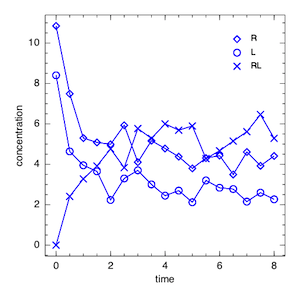
# FramedPlot can be used for plotting a single plot
p = FramedPlot("xlabel","time")
setattr(p,"ylabel","concentration") # attributes can be changed with setter functions 
# similar to MATLABs `set` and `get`

# building a plot using Winston is like composing a collage:
# build one element after the other
# then add it all to the canvas (the FramedPlot)
r = Points(time,R,"type","diamond", "color","blue")
l = Points(time,L,"type","circle", "color","blue")
rl = Points(time,RL,"type","cross", "color","blue")

cr = Curve(time,R, "color","blue")
cl = Curve(time,L, "color","blue")
crl = Curve(time,RL, "color","blue")

setattr(r,"label","R")
setattr(l,"label","L")
setattr(rl,"label","RL")
lgnd = Legend(.8,.9,{r,l,rl})

# adding does not! need to be done at the end
add(p,r,l,rl,cr,cl,crl,lgnd)
# Winston/ijulia do not yet support the display of the generated plots,
# but it is possible to save the plot to a file 
# eps, png and svg are supposed to be supported, but 
# svg did not work on my machine out of the box
file(p,"julia_rlbinding.png")

I have to say, I like the way Winston/julia approach graphics. It requires a few more steps than the plot function in MATLAB, but it is also more consistent. The post got longer than expected, hence I moved the treatment of subplots to the next post.

Update

Steven G. Johnson pointed out in the julia-user mailing list that pyplot (a matplotlib wrapper) is another, fourth way for plotting in julia. Looks quite MATLAB-like at a first glance.

Any comments/questions? Send me an email.